
Two batters in a school cricket team each average 30 runs over eight innings. Aarav scored 28, 31, 30, 29, 32, 30, 31 and 29. Bibek scored 0, 72, 5, 64, 3, 55, 1 and 40. (The scores are made up, to make the point.) The same average, but you know at once that they are very different players: Aarav gets about 30 every time, and Bibek either wins the match or is out in the first over.
So here is this unit’s question: how do you put a number on how spread out the values are, and use it to say which set is steadier? The answer, the standard deviation, comes out at about 1 run for Aarav and 29 runs for Bibek. Exam boards, weather offices, factories and banks use the same number every day.
11.1 Introduction
Statistics is the branch of mathematics that collects data, presents it, analyses it and draws conclusions from it. It is as old as government: the rulers of Babylonia, Egypt and China counted their people, their land and their harvests to plan taxes and armies. The word itself comes from state.
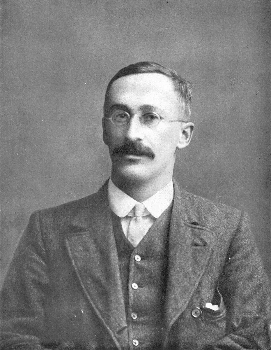
In the twentieth century statistics became a science of its own. Sir Ronald A. Fisher (1890–1962) laid much of the foundation of modern statistics, and is often called its father; Karl Pearson (1857–1936) and William Sealy Gosset (1876–1937) made other great contributions, and you will meet all three in this unit. Today, with computers and huge amounts of data, statistics is used in almost every field: medicine, farming, sport, weather, business and the artificial intelligence on your phone.
Dispersion
When you study a set of data, you usually begin with a measure of central tendency, the mean, median or mode, which you met in Grade 10 Math. It gives one value for the center of the data. But the center alone doesn’t tell the whole story. Look at the marks of five students in each of three groups:
| Group | Marks | Mean | ||||
|---|---|---|---|---|---|---|
| A | 48 | 49 | 50 | 51 | 52 | 50 |
| B | 40 | 45 | 50 | 55 | 60 | 50 |
| C | 20 | 35 | 50 | 65 | 80 | 50 |
All three groups have a mean of 50, but:
- in group A (low variation), every mark is within 2 of the mean: the students did almost equally well;
- in group B (moderate variation), the marks are spread out a moderate distance from the mean;
- in group C (high variation), the marks are widely spread: some students did very well and some poorly.
Looking only at the mean, you would think the three groups did the same. What makes them different is their spread.
Dispersion (or variation) is how far the values of a data set differ from one another, or from their central value. A measure of dispersion is a number that says how spread out the values are.
Measures of dispersion help us:
- a.to decide whether the data are consistent (steady) or variable;
- b.to compare how reliable two or more data sets are;
- c.to check how well the mean, median or mode represents the data: the smaller the spread, the better one central value describes every value;
- d.to make decisions in education, business, economics and science (which supplier’s parts are more uniform, which medicine works more reliably, which investment is less risky).
The central value describes the middle of the data; the dispersion describes its spread. To understand a data set you need both.
The simplest measure of dispersion is the range, the highest value minus the lowest: 4 for group A, 20 for B and 60 for C. But the range uses only the two end values, and one unusual value changes it completely. This unit builds three better measures: the quartile deviation, the mean deviation and the standard deviation.
Two classes took the same test. Both had a mean of 62 marks. In class P the marks ranged from 55 to 70; in class Q from 20 to 98. Which statement is right?
Pick an answer to see why.
11.2 Quartile deviation
Each class includes its lower limit and goes up to, but not including, its upper limit. The class 55–60 kg holds 55, 56, 56.5, 57, 58, 59 and 59.5, but not 60, which belongs to the next class, 60–65.
Data that can take any value in a stretch, decimals as well as whole numbers (heights, weights, times), grouped into classes like these, form a continuous series.
11.3 Quartile deviation of a continuous series
You met the quartiles in Grade 10 Math. They cut the data, in order, into four quarters:
- the first quartile Q₁ has 25% of the data below it and 75% above;
- the second quartile Q₂, the median, has 50% below and 50% above;
- the third quartile Q₃ has 75% below and 25% above.
So the middle half of the data lies between Q₁ and Q₃. The width of that middle half is the interquartile range:
Half of the interquartile range is the quartile deviation (Q.D.), also called the semi-interquartile range:
The quartile deviation has the data’s own unit (marks, kg, rupees), so it can’t compare data in different units, or data of very different sizes. For that we divide by Q₃ + Q₁ and get a pure number, the coefficient of quartile deviation:
The quartile deviation ignores the lowest quarter and the highest quarter of the data. That is its weakness (it uses only half the data) and its strength: one very high or very low value can’t change it, and it can be found even when the first or last class is open-ended (“less than 20”, “60 or more”), where the mean can’t.
To find Q₁ and Q₃ of a continuous series, as in Grade 10 Math:
- Make the cumulative frequency (cf) table. Its last cf is N.
- Q₁ is the th item; Q₃ the th.
- The quartile’s class is the first whose cf reaches that position.
- Then
where L is the lower limit of the quartile’s class, cf the cumulative frequency of the class before it, f the frequency of the quartile’s class and h its width. (Some books write l and i for L and h.)
Worked examples
Exercise 11.1
Question 1
A. What is another name for the quartile deviation?
Pick an answer to see why.
B. What percentage of the data lies between the two quartiles that the quartile deviation is built from?
Pick an answer to see why.
C. Which formula gives the quartile deviation?
Pick an answer to see why.
D. If Q₁ = 10 and Q₃ = 30, what is the quartile deviation?
Pick an answer to see why.
E. Which values are left out when the quartile deviation is calculated?
Pick an answer to see why.
F. If the quartile deviation is 10 and the upper quartile is 30, what is the lower quartile?
Pick an answer to see why.
Question 2
Find the quartile deviation and the coefficient of quartile deviation.
| Marks | 0–10 | 10–20 | 20–30 | 30–40 | 40–50 |
|---|---|---|---|---|---|
| Students | 4 | 10 | 20 | 10 | 6 |
Answer
| Wages (Rs thousand) | 0–5 | 5–10 | 10–15 | 15–20 | 20–25 | 25–30 |
|---|---|---|---|---|---|---|
| Workers | 4 | 6 | 3 | 8 | 12 | 7 |
Answer
| Weight (kg) | 20–30 | 30–40 | 40–50 | 50–60 | 60–70 | 70–80 | 80–90 |
|---|---|---|---|---|---|---|---|
| Students | 4 | 5 | 10 | 15 | 8 | 7 | 1 |
Answer
| Marks | 0 ≤ x < 10 | 10 ≤ x < 20 | 20 ≤ x < 30 | 30 ≤ x < 40 | 40 ≤ x < 50 |
|---|---|---|---|---|---|
| Students | 5 | 10 | 15 | 10 | 5 |
Answer
| Marks (less than) | 20 | 30 | 40 | 50 | 60 |
|---|---|---|---|---|---|
| Students | 5 | 12 | 27 | 40 | 50 |
Answer
| Wages per hour (Rs, more than) | 100 | 200 | 300 | 400 | 500 |
|---|---|---|---|---|---|
| Workers | 100 | 80 | 60 | 40 | 20 |
Answer
Question 3
The marks of 30 students in mathematics are:
| 12 | 25 | 36 | 45 | 18 | 22 | 33 | 54 | 42 | 29 |
| 38 | 41 | 15 | 20 | 48 | 52 | 30 | 24 | 19 | 37 |
| 44 | 21 | 35 | 40 | 14 | 26 | 49 | 31 | 23 | 50 |
Taking the first class as 10–20, make a frequency table.
Answer
Find the first quartile.
Answer
Find the third quartile.
Answer
Find the quartile deviation.
Answer
Find the coefficient of quartile deviation.
Answer
11.4 Mean deviation
The quartile deviation looks at only two values. A measure that uses every value asks: on average, how far is each value from the center?
The mean deviation (MD) is the mean of the distances of the values from a central value, the mean or the median (sometimes the mode). A distance is never negative: 5 below the mean and 5 above it are both 5 away. So each difference is taken as its absolute value, |m − X|, the difference without its sign. (Without the bars, the differences from the mean always add up to exactly 0, the reason the mean is the balance point.)
For a continuous series, with mid-values m:
Writing D for the difference, both are . For a list of values, the mean deviation from the median is never bigger than the one from the mean, because the median is the point from which the total distance is least. In a grouped table the two are usually equal or nearly so, as above.
Worked examples
Exercise 11.2
Question 1
A. Which formula gives the mean deviation?
Pick an answer to see why.
B. If all the values of a data set are equal, what is the mean deviation?
Pick an answer to see why.
C. Which central value can the mean deviation be calculated from?
Pick an answer to see why.
D. If , N = 30 and the mean is 40, what is the coefficient of mean deviation?
Pick an answer to see why.
Question 2
Find the mean deviation from the mean, and its coefficient.
| Weight (kg) | 0–4 | 4–8 | 8–12 | 12–16 | 16–20 | 20–24 |
|---|---|---|---|---|---|---|
| Children | 7 | 7 | 10 | 15 | 7 | 6 |
Answer
| Marks | 0–10 | 10–20 | 20–30 | 30–40 | 40–50 | 50–60 |
|---|---|---|---|---|---|---|
| Students | 8 | 12 | 20 | 40 | 12 | 8 |
Answer
Question 3
Find the mean deviation from the median, and its coefficient.
| Weight (kg) | 20–30 | 30–40 | 40–50 | 50–60 | 60–70 | 70–80 |
|---|---|---|---|---|---|---|
| Students | 7 | 12 | 18 | 28 | 16 | 14 |
Answer
| Weight (kg) | 3–5 | 5–7 | 7–9 | 9–11 | 11–13 |
|---|---|---|---|---|---|
| Dogs | 1 | 4 | 6 | 4 | 1 |
Answer
Question 4
A school held a mathematics test of 50 full marks. The marks of 10 students are:
| Marks | less than 10 | less than 20 | less than 30 | less than 40 | less than 50 |
|---|---|---|---|---|---|
| Students | 1 | 3 | 7 | 9 | 10 |
Find the mean deviation from the mean and its coefficient.
Answer
Find the mean deviation from the median and its coefficient.
Answer
Questions 5 and 6
In a factory, the workers’ hourly wages range from Rs 100 to under Rs 800. Find the mean deviation from the mean and its coefficient.
| Wages per hour (Rs) | Workers |
|---|---|
| more than 100 | 60 |
| more than 200 | 56 |
| more than 300 | 50 |
| more than 400 | 40 |
| more than 500 | 20 |
| more than 600 | 10 |
| more than 700 | 4 |
Answer
The marks of 28 Grade 10 students in mathematics are:
| 15 | 62 | 50 | 70 | 74 | 34 | 60 |
| 41 | 14 | 48 | 28 | 38 | 64 | 21 |
| 57 | 40 | 34 | 30 | 47 | 20 | 75 |
| 45 | 56 | 29 | 22 | 13 | 53 | 66 |
- a.Make a frequency table with the first class 10–20.
- b.Find the mean deviation from the mean and its coefficient.
- c.Find the mean deviation from the median and its coefficient.
Hint
Answer
11.5 Standard deviation
Here this section is 11.5, its subsections 11.5.1 to 11.5.4, and the box plot 11.6; some editions number them differently.
The mean deviation got rid of the minus signs by ignoring them. The standard deviation gets rid of them by squaring: a square is never negative. Then, to get back to the data’s own unit (marks, not marks²), it takes the square root at the end.
The standard deviation is the square root of the mean of the squared distances of the values from their mean. It is written , the small Greek letter sigma:
The square of the standard deviation, , is called the variance.
Of all the measures of dispersion, the range, the quartile deviation, the mean deviation and the standard deviation, the standard deviation is the most widely used and the most reliable.
In the next drawing, each mark has a stem from the mean (the red line): the stems are the distances. MD is the stems’ average length; is the square root of the average of their squares. Try the groups of 11.1, then pull one mark far away and watch pull ahead of MD.
11.5.1 Uses of standard deviation
The standard deviation is used wherever it matters how steady something is:
- a.Education: to compare how consistent the results of students, classes or schools are.
- b.Weather: to measure how much the temperature or rainfall of a place varies from year to year.
- c.Investment: a share whose price has a large standard deviation is riskier.
- d.Quality control: a factory measures its products (the weight of a packet of noodles, the length of a bolt) and checks that their standard deviation stays small, so the quality is uniform.
11.5.2 Coefficient of standard deviation
The standard deviation has the data’s own unit. To compare spreads in different units (heights in cm and weights in kg), or of data of very different sizes, divide it by the mean:
where is the standard deviation and X the mean. The smaller the coefficient, the more uniform (stable, consistent) the data; the larger, the more variable.
11.5.3 Coefficient of variation
The coefficient of standard deviation is usually less than 1, so for everyday use it is turned into a percentage. The coefficient of variation (C.V.) is the coefficient of standard deviation as a percentage:
As with the coefficient: the smaller the C.V., the more uniform the data; the larger, the more variable. It is the standard way to say which of two sets is more consistent. (It can be more than 100% when the values are very spread out compared with their mean: Bibek’s scores in the opening come close.)
Two rice mills fill 25 kg sacks. Mill P’s sacks have a mean of 25.2 kg and a standard deviation of 0.4 kg; mill Q’s a mean of 25.0 kg and a standard deviation of 0.1 kg. Which is right?
Pick an answer to see why.
11.5.4 Standard deviation of a continuous series
In a continuous series each class is represented by its mid-value m, and each squared distance is counted f times. There are four ways of working it out. They give the same answer; choose the one that keeps the numbers easiest.
The actual mean method
where m is the mid-value, and X the mean. The steps:
- a.Find the mid-value m of each class.
- b.Find fm for each class and their sum .
- c.Find the mean .
- d.Find each class’s distance from the mean, m − X, and square it.
- e.Multiply each square by f: .
- f.Add these up: .
- g.Put the sums into formula (i).
This method is easiest when the mean is a whole number.
The direct method
Opening the bracket in (i) gives a formula that needs no distances at all, only and :
“The mean of the squares minus the square of the mean.” The steps:
- a.Find the mid-value m.
- b.Find fm for each class.
- c.Find for each class (m × fm is quickest).
- d.Find and .
- e.Put them into formula (ii).
It suits small mid-values, when the mean is not a whole number.
The short-cut (assumed mean) method
Choose a mid-value near the middle as an assumed mean A, and use the distances from it, d = m − A:
The steps:
- a.Find the mid-value m.
- b.Choose a mid-value as A and find d = m − A.
- c.Find fd for each class.
- d.Find for each class (d × fd).
- e.Find and .
- f.Put them into formula (iii).
Moving every value by the same amount doesn’t change the spread, so the standard deviation of the d’s is the standard deviation of the m’s. That is why the method works. It is useful when the actual mean is an awkward decimal.
The step deviation method
When the classes are wide and the numbers large, divide the distances by the class width h as well: , small whole numbers like −2, −1, 0, 1, 2. Then multiply the answer by h to get back to the data’s unit:
The steps:
- a.Find the mid-value m.
- b.Choose a mid-value as A and find .
- c.Find fd′ for each class.
- d.Find for each class (d′ × fd′).
- e.Find and .
- f.Put them into formula (iv).
Back to the batters
The two batters of the opening both average 30 runs. With the standard deviation:
| Batter | Scores | Mean | C.V. | |
|---|---|---|---|---|
| Aarav | 28, 31, 30, 29, 32, 30, 31, 29 | 30 | 1.22 | 4.1% |
| Bibek | 0, 72, 5, 64, 3, 55, 1, 40 | 30 | 29.03 | 96.8% |
Aarav’s squared distances from 30 add up to 12, so ; Bibek’s add up to 6740, so . Aarav is about 24 times as consistent. A captain who needs a steady 30 sends in Aarav; one who needs a big score to win, and can risk a duck, might choose Bibek. Statistics gives the numbers; the decision still depends on the match.
Exercise 11.3
Question 1
A. What is the standard deviation?
Pick an answer to see why.
B. Which formula gives the coefficient of variation?
Pick an answer to see why.
C. If the variance of a data set is , what is the standard deviation?
Pick an answer to see why.
D. One data set has a higher coefficient of variation than another. Compared with the other, it is:
Pick an answer to see why.
E. If and N = 100, what is the standard deviation?
Pick an answer to see why.
Question 2
What is the standard deviation?
Answer
What is the coefficient of variation?
Answer
How is the mean deviation different from the standard deviation?
Answer
How is the coefficient of standard deviation different from the coefficient of variation?
Answer
Question 3
If N = 100, and , find the mean and the standard deviation.
Answer
If N = 40, and , where d = m − A for an assumed mean A, find the standard deviation.
Answer
Question 4
Find the standard deviation and its coefficient.
| Weight (kg) | 10–20 | 20–30 | 30–40 | 40–50 | 50–60 |
|---|---|---|---|---|---|
| Students | 5 | 10 | 12 | 7 | 6 |
Answer
| Marks | 10–20 | 20–30 | 30–40 | 40–50 | 50–60 | 60–70 |
|---|---|---|---|---|---|---|
| Students | 8 | 12 | 15 | 20 | 12 | 8 |
Answer
| Weight (kg) | 3–5 | 5–7 | 7–9 | 9–11 | 11–13 |
|---|---|---|---|---|---|
| Dogs | 1 | 3 | 5 | 4 | 2 |
Answer
Question 5
The marks of 40 students in a mathematics exam of 50 full marks are:
| Marks | less than 10 | less than 20 | less than 30 | less than 40 | less than 50 |
|---|---|---|---|---|---|
| Students | 5 | 11 | 25 | 35 | 40 |
Find the mean mark.
Answer
Find the standard deviation and its coefficient.
Answer
Question 6
In a factory, the daily wages of the workers range from Rs 600 to over Rs 1,200:
| Daily wage (Rs) | Workers |
|---|---|
| more than 600 | 100 |
| more than 700 | 80 |
| more than 800 | 55 |
| more than 900 | 25 |
| more than 1000 | 15 |
| more than 1100 | 8 |
| more than 1200 | 4 |
Find the mean wage.
Answer
Find the standard deviation and its coefficient.
Answer
Find the variance.
Answer
Find the coefficient of variation.
Answer
Question 7
The monthly salaries of the workers in two shoe factories are:
| Factory A | Factory B | |
|---|---|---|
| Workers | 40 | 50 |
| Mean monthly salary | Rs 35,000 | Rs 45,000 |
| Standard deviation | Rs 40 | Rs 35 |
Which factory spends more on salaries?
Answer
Which factory’s salaries are more uniform? Give a reason.
Answer
Question 8
The scores of 36 Grade 10 students in a mathematics exam are:
| 35 | 62 | 72 | 50 | 70 | 74 | 34 | 60 | 36 |
| 21 | 14 | 75 | 48 | 28 | 38 | 64 | 21 | 45 |
| 57 | 40 | 19 | 34 | 30 | 47 | 20 | 75 | 51 |
| 45 | 56 | 22 | 29 | 22 | 13 | 53 | 66 | 62 |
Make a frequency table with the first class 10–20.
Answer
Find the mean score.
Answer
Find the standard deviation and its coefficient.
Answer
Find the coefficient of variation.
Answer
11.6 Whisker box plot
A mean, or even a mean and a standard deviation, can hide what the data really look like. A whisker box plot (box-and-whisker plot) draws the whole spread in one picture, and puts two data sets side by side so they can be compared at a glance. You met it in Grade 9.
A whisker box plot shows a data set by its five-number summary: the smallest value (minimum), the first quartile, the median, the third quartile and the largest value (maximum). The box, from Q₁ to Q₃, holds the middle 50% of the data; the two whiskers, from the smallest value to Q₁ and from Q₃ to the largest, hold the lowest and the highest 25% each.
Read it like this:
- the line inside the box is the median, the typical value;
- the width of the box is the interquartile range, Q₃ − Q₁: a narrow box means consistent data;
- the whole width, whisker end to whisker end, is the range;
- a long whisker on one side means the data stretch far that way: a few values much higher (or lower) than the rest.
In Activity 1, half of the students are between 114 and 145 cm, and the median, 126 cm, is nearer the bottom of the box than the top: in the middle half, the heights above the median are more spread out than those below it.
Steps to draw a whisker box plot:
- Arrange the data in ascending order.
- Find the smallest value, Q₁, the median, Q₃ and the largest value. For n values in order, Q₁ is the th, the median the th and Q₃ the th, as in Grade 10 Math.
- Draw a scale and mark the five values on it.
- Draw a box from Q₁ to Q₃ with a line across it at the median, then the whiskers from the smallest value to Q₁ and from Q₃ to the largest.
11.6.1 Comparing two data sets with box plots
To compare two data sets with box plots, draw them on one scale and compare:
- the medians, for which is higher in a typical case;
- the boxes’ widths (interquartile ranges), for which is more consistent;
- the whiskers, for the extremes: the guaranteed minimum, the best case.
In two box plots on one scale, plot P’s box runs from 40 to 48 and plot Q’s from 30 to 65. Both medians are 44. What can you say?
Pick an answer to see why.
Exercise 11.4
Question 1
The batteries of two brands of mobile phone were tested to see how long they last after a full charge.
A. On the basis of the median, which brand’s battery lasts longer in general?
Pick an answer to see why.
B. Which brand’s battery life is more consistent?
Pick an answer to see why.
C. Which brand has the higher guaranteed minimum battery life?
Pick an answer to see why.
D. What does the red line in each box show?
Pick an answer to see why.
Question 2
The yield of paddy from a field over ten years with two fertilizers, A and B:
With which fertilizer is the lowest yield higher?
Answer
If you were a farmer who wanted to keep the risk small, which fertilizer would you choose, and why? (Hint: look at the interquartile ranges.)
Answer
Was there a year when Fertilizer B gave an unusually high yield? How does the plot show it?
Answer
Question 3
The life of two kinds of battery:
What is the median life of Battery A?
Answer
What is the median life of Battery B?
Answer
Find the range of each battery’s life.
Answer
Which battery would you buy? Give reasons.
Answer
Question 4
The numbers of mobile phones sold by two shops over one week are:
| Shop | Mon | Tue | Wed | Thu | Fri | Sat | Sun |
|---|---|---|---|---|---|---|---|
| A | 8 | 5 | 14 | 9 | 11 | 7 | 18 |
| B | 10 | 12 | 8 | 16 | 6 | 3 | 2 |
Find the five-number summary of each.
Answer
Draw the two box plots.
Answer
Compare the shops by their medians and interquartile ranges.
Answer
How the SEE asks it
In the SEE’s Optional Mathematics paper (75 marks, 3 hours), Statistics is a content area of its own. CDC’s specification grid gives it 7 marks, in three kinds of question:
| Group | Kind of question | Statistics’ marks | Levels |
|---|---|---|---|
| A | multiple choice, 1 mark | 1 | understanding 1 |
| B | within the content area: one question on statistics alone, in three 1-mark parts | 3 | knowledge 1, understanding 1, higher ability 1 |
| C | across content areas: parts of a longer question joining statistics with another area | 3 | application 3 |
In CDC’s model paper, statistics turns up in all three groups: what a higher coefficient of variation means (group A, 1 mark); two box plots on one scale, read for the median, then a coefficient of quartile deviation, then a choice between the two data sets with a reason (group B, 1 + 1 + 1); and, inside a question that goes on to continuity, the coefficient of variation from a grouped table (group C, 3 marks).
What each kind asks, and where its marks are:
- 1-mark questions: what Q.D., MD, , variance or C.V. means; “smaller C.V., more uniform”; from the variance; Q.D. from Q₁ and Q₃. Work them on rough paper.
- Knowledge: a formula written exactly, or a value read off a box plot (a median, a quartile, the smallest value).
- Understanding: a coefficient from given values, or .
- Higher ability: a choice with a reason drawn from the numbers: the narrower box or the smaller C.V. is more consistent; the higher minimum is safer.
- Application (group C): the full table, m, fm, (or d, fd, ), then X, and C.V. Write the table neatly: most of the marks are in it.
Here is a question in the style of group B, written for this book, with how it is marked.
Miscellaneous exercise
These questions join the unit’s measures together, as the SEE’s longer statistics questions do.
The marks of the students in an exam are:
| Marks | 20–30 | 30–40 | 40–50 | 50–60 | 60–70 | 70–80 | 80–90 |
|---|---|---|---|---|---|---|---|
| Students | 4 | 6 | 10 | 17 | 11 | 9 | 3 |
- a.Write the relation between the quartile deviation, Q₁ and Q₃.
- b.Find the standard deviation.
- c.Find the coefficient of variation.
Answer
The marks of 40 students in a second-term mathematics exam are:
| Marks | 20–30 | 30–40 | 40–50 | 50–60 | 60–70 | 70–80 |
|---|---|---|---|---|---|---|
| Students | 5 | 9 | 12 | 7 | 4 | 3 |
- a.Write the formula for the mean deviation from the mean.
- b.Find the standard deviation.
- c.The standard deviation of the first-term marks was 8.75. Compare the two terms’ marks.
Answer
The monthly salaries of 50 employees of a bank are:
| Salary (Rs) | more than 20,000 | more than 30,000 | more than 40,000 | more than 50,000 | more than 60,000 | more than 70,000 |
|---|---|---|---|---|---|---|
| Employees | 50 | 45 | 25 | 9 | 4 | 2 |
- a.What is the quartile deviation?
- b.Which measure of dispersion suits this data? Give a reason.
- c.Find the quartile deviation and its coefficient.
Answer
The marks of 40 students in a mathematics exam are:
| 75 | 35 | 45 | 47 | 60 | 61 | 56 | 39 | 56 | 52 |
| 42 | 60 | 69 | 42 | 43 | 46 | 55 | 56 | 35 | 51 |
| 58 | 61 | 49 | 57 | 51 | 59 | 47 | 52 | 57 | 55 |
| 48 | 58 | 54 | 67 | 46 | 56 | 39 | 48 | 51 | 60 |
- a.Write the formula for the coefficient of variation.
- b.Make a frequency table with classes 5 marks wide.
- c.Find the coefficient of variation.
- d.The coefficients of variation of two students’ results, A and B, were 21% and 12%. Whose results are more consistent? Why?
Answer
The marks of 11 Grade 10 students in mathematics and science are:
Mathematics: 20, 93, 44, 58, 64, 68, 75, 82, 87, 23, 98
Science: 65, 19, 25, 31, 38, 45, 57, 35, 71, 15, 80
- a.Find the five-number summary of each.
- b.Draw both box plots on one scale.
- c.In which subject are the marks more consistent? Give a reason.
Answer
Practice every question in the book, and keep track of the ones you miss →
Where these facts come from
- John Graunt (1620–1674), a haberdasher; Natural and Political Observations Made upon the Bills of Mortality (1662); his doubts about the plague figures; the first life table; regarded as the founder of demography (11.1): Wikipedia, “John Graunt”, read October 2026.
- The bills of mortality, weekly lists of burials (and christenings) in London’s parishes (11.1): Wikipedia, “Bills of mortality”, read October 2026.
- Ronald Fisher as a founder of modern statistics; his introduction of the word variance (1918) (11.1, 11.5): Wikipedia, “Ronald Fisher” and “Variance”, read October 2026.
- Karl Pearson’s first written use of “standard deviation”, in 1894 (11.5): Wikipedia, “Standard deviation”, History, read October 2026.
- William Sealy Gosset at Guinness, his two terms in Pearson’s laboratory in 1906–07, the pen name “Student”, “The probable error of a mean” in Biometrika (1908), the photograph of 1908 (11.5): Wikipedia, “William Sealy Gosset”, read October 2026; Student’s t-test and its use for small samples: Wikipedia, “Student’s t-test”, read October 2026.
- The box plot, introduced by John Tukey in 1970 and in Exploratory Data Analysis (1977), after Mary Eleanor Spear’s range bars of 1952 (11.6): Wikipedia, “Box plot”, read October 2026; Tukey and the word “bit”: Wikipedia, “John Tukey”, read October 2026.
- The photo of Gosset: its Wikimedia Commons file page.
- The batters, the buses, the rice mills, the shops and the health post in the examples are made up, to show the methods.
- CDC’s specification grid and model paper for Optional Mathematics, 2082 (How the SEE asks it): the textbook folder,
Specification Grids/grid-Opt. Math-G10.
A companion to your textbook, not a replacement for it: study from the book your school uses, and where the two differ, follow your teacher. Found a mistake? Please tell us.