Does Ice Cream Cause Drowning?

A graph like Sabina’s, one dot for each case with two measurements as its coordinates, is a scatter graph (or scatter plot). Read it as a shape. Her dots run from the bottom left to the top right: months with more ice cream tend to have more drownings. When one thing tends to be bigger where the other is bigger, the two have a positive association. If the dots ran from top left to bottom right (the more of one, the less of the other), it would be negative.

Then ask how tight it is: dots close along a line make a strong association; Sabina’s broad band is moderately strong. Ask whether the band is straight (linear) or bends, and look for clusters (groups with gaps between them) and outliers, dots far from all the others.

“Moderately strong” is a judgment by eye. Statisticians measure it with one number, the correlation coefficient r. To see where it comes from, draw two dashed lines through the dots: one at the average of the x-values, one at the average of the y-values. They meet at the point of averages and cut the graph into four corners.

A dot in the top right corner is above average in both. A dot in the bottom left is below average in both. Both kinds are evidence of “together”. A dot in the top left or bottom right goes against it: one measurement is above average and the other below.

Now give each dot a rectangle, from the point of averages to the dot. Its width is how far the dot is from the average across, $x - \bar{x}$, and its height how far from the average up, $y - \bar{y}$ (the bar means “the average of”). In the two rising corners the two distances have the same sign, so their product is positive: color those rectangles blue. In the falling corners the product is negative: red.

Add up the blue areas and take away the red ones: that sum, $\sum (x - \bar{x})(y - \bar{y})$, is big and positive when most dots are in the rising corners, big and negative when most are in the falling ones, and near zero when they balance. It can’t be used as it is, though: measure the ice cream in single cups instead of thousands and every rectangle becomes a thousand times wider. So it is divided by a number with the same units, made from how spread out each measurement is on its own:

$$r = \frac{\sum (x - \bar{x})(y - \bar{y})}{\sqrt{\sum (x - \bar{x})^2 \times \sum (y - \bar{y})^2}}$$

This is Pearson’s correlation coefficient, the one Grade 12 maths calculates “by Karl Pearson’s method”. It has no units, and it is always between −1 and +1:

• +1: every dot exactly on a rising straight line; −1: every dot on a falling one;
• near 0: no straight-line pattern;
• in between, how close the dots come to a line. Sabina’s 36 months give r = 0.78.

The line of best fit

In the widget above, press Best-fit line. The green line always passes through the point of averages, and it is tilted so that the dots are as close to it, up and down, as they can be. (Its slope is the blue area minus the red divided by $\sum (x - \bar{x})^2$.) Worked out for Sabina’s 36 months, the line says: for every thousand more cups of ice cream sold, about 0.73 more drownings.

That is a perfectly good prediction: told only that a month sold 15 thousand cups, you would bet on a busy month for the rescue teams, and usually be right. What the line can’t tell you is what would happen if somebody changed the ice cream sales. Predicting and changing are different questions. (And a line only describes the range of its dots: Sabina has no month with 30 thousand cups, so it says nothing about one.)

Now color Sabina’s months by how hot they were: the average of each day’s highest temperature in that month.

All 36 months together give r = 0.78. But take only the hot months: they all had plenty of drownings, between 7 and 15, and the ones with the most ice cream didn’t have more. Within the hot months r is −0.01; within the warm months −0.10; within the cool months 0.15. Once you compare months that were equally hot, the pattern is gone.

So the heat is behind both. It sends people to the ice cream shop, and it sends them into the water. Something that drives both of two measurements, and so makes them move together, is called a confounding variable (or a lurking variable, when nobody measured it). In made-up numbers the hidden cause can be known for sure; in real data it rarely is, and some confounders are never measured at all.

Holding the third thing fixed, as you just did by comparing months of the same heat, is the first test to try on any surprising correlation. It is not foolproof: it only works for the third things you thought of and measured. And sometimes splitting into groups can even reverse a pattern: that is Simpson’s paradox, the topic Can a Treatment Win in Every Group but Lose Overall?

The ice cream is one way two things can move together without one causing the other. When you meet a correlation, run through all four:

1. One causes the other. Hot weather really does make people buy ice cream: a cool, rainy Jestha would sell less. This is the case everyone jumps to.
2. The other way round. Suppose the beaches and river banks with the most lifeguards also have the most drownings. That doesn’t mean lifeguards cause drowning: lifeguards are sent to the places where people drown. The cause runs the other way, which is called reverse causation.
3. Something behind both, a confounding variable, as with the heat.
4. Chance. Two things can go together by pure luck, and the more pairs anyone looks at, the more such lucky pairs turn up.

The fourth is the one people forget. In 2014 Tyler Vigen began publishing what he called spurious correlations, found by comparing thousands of series of numbers with each other. One from his first collection: from 1999 to 2009, the number of people in the United States who drowned by falling into a swimming pool went up and down with the number of films the actor Nicolas Cage appeared in, with r = 0.67. Nobody thinks his films push people into pools.

How lucky is that? A computer can find out by making up pairs of unrelated lists of 11 random numbers, as many as you like, and working out r for each. About 2.5% of the pairs reach Vigen’s 0.666 or more (either way, up or down) by chance alone. That sounds rare until you see how many pairs there are. Take 100 lists: that is 100 × 99 ÷ 2 = 4{,}950 pairs, so about 125 pairs as “strong” as Vigen’s, every one of them meaningless. Look at thousands of lists, as he did, and impressive correlations are guaranteed.

In 1973 the statistician Frank Anscombe published four small sets of numbers, 11 points each, to argue that every set of data should be drawn before it is calculated. The four have the same averages, the same r, 0.816, and the same line of best fit, y = 3 + 0.5x.

Only the first is what r = 0.816 makes you imagine. The second is a smooth curve, a perfect relationship that a straight line describes badly. The third is a perfect straight line with one point knocked off it; without that point, r would be 0.99999, as near 1 as makes no difference. The fourth has no pattern at all: ten points in one column, where x tells you nothing about y, and one far point that creates the whole correlation by itself.

Try the last trick in the widget above: start from Far point. Seven points in a shapeless huddle and one far away give r = 0.93; drag the far point down into the middle of the huddle and r falls to about 0.14. One unusual case, a typing mistake or an exceptional month, can make or break a correlation. So: draw the dots first, then believe the number.

If correlation can’t show a cause, what can? The strongest answer is to stop watching and start doing: change the thing yourself, for some people and not others, and see what happens. But it has to be done fairly.

Suppose a company sells a tonic it says keeps children from falling ill. One way to test it is to compare the children whose families bought it with those whose families didn’t. Here the widget knows something you usually can’t: which children are well fed.

Start with Families choose and a tonic that does nothing. The tonic’s group falls ill about half as often (on average 17% against 32%; each run wobbles a little): it looks like a wonder. Now press Show who is well fed. The families who bought the tonic were mostly the better-off ones: about 78% of the tonic group were well fed, against 27% of the others. Good food did it all. The confounding variable sneaked in through who chose the treatment.

Now switch to Toss a coin. A coin doesn’t know who is well fed, so each group gets about half of each kind, and both fall ill about 25% of the time. Make the tonic work and the gap that appears, about 12.5% against 25%, is the tonic’s own. The coin balances every other difference between the children too, including the ones nobody has thought of. That is its whole point.

A study where the people are put into groups by chance, one group given the treatment and the other not, is a randomized controlled experiment (in medicine, a randomized controlled trial). The group without the treatment is the control group. A study that only watches what people do anyway, like Sabina’s months or families choosing a tonic, is an observational study. A survey, a third kind, asks or measures a sample to describe a whole population; the topic Can 1,000 People Speak for 3 Crore? is about getting that right. Only the experiment, with its coin, can show a cause on its own.

When an experiment would be wrong or impossible, you can’t randomize. Nobody may make a thousand children smoke to see what happens. Then scientists have to build the case from observational studies, carefully, and that is what happened with cigarettes.

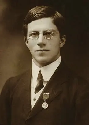
Hill’s viewpoints are still how epidemiologists judge a cause when no experiment can be done: a strong association, found again by different people in different places; the cause coming first; more of the cause giving more of the effect; a way it could work. None is proof alone. Together they made the case against cigarettes. Today the World Health Organization estimates that tobacco kills more than 7 million people a year.

• Can a Treatment Win in Every Group but Lose Overall? Simpson’s paradox: when a hidden third thing turns a pattern upside down.
• Can 1,000 People Speak for 3 Crore? Surveys, samples and the margin of error.
• Is a Positive Test Result Bad News? Conditional probability and base rates, the other great trap in reading medical numbers.
• Can a Graph Lie? (Grades 6–8) Honest and misleading charts of the same data.
• What Does an Average Hide? (Grades 6–8) Means, medians and the spread an average leaves out.
• Grade 10 Math: Statistics, averages of grouped data, the tools under every scatter graph; and Grade 10 Computing: Data Science, charts of many variables and drawing honest conclusions from them in Python.